Observing the Summer Triangle#
Note
Your calculated rise/set and other times may differ slightly from those in this tutorial, on the order of ~1 second. This is a normal variance in precision due to several factors, including varying IERS tables and machine architecture.
Contents#
Defining Objects#
Say we want to look at the Summer Triangle (Altair, Deneb, and Vega) using the Subaru Telescope.
First, we define our Observer object:
>>> from astroplan import Observer

>>> subaru = Observer.at_site('subaru')
Then, we define our FixedTarget’s, since the Summer Triangle is
fixed with respect to the celestial sphere (if we ignore the relatively small
proper motion). We will use the from_name class method,
which queries the CDS name resolver for your target’s coordinates (giving you
the power of SIMBAD!):
>>> from astropy.coordinates import SkyCoord
>>> from astroplan import FixedTarget

>>> altair = FixedTarget.from_name('Altair')
>>> vega = FixedTarget.from_name('Vega')
For objects that can’t be resolved with from_name, you
can enter coordinates manually:
>>> coordinates = SkyCoord('20h41m25.9s', '+45d16m49.3s', frame='icrs')
>>> deneb = FixedTarget(name='Deneb', coord=coordinates)
We also have to define a Time (in UTC) at which we wish to
observe. Here, we pick 2AM local time, which is noon UTC during the
summer:
>>> from astropy.time import Time

>>> time = Time('2015-06-16 12:00:00')
Observable?#
Next, it would be handy to know if our targets are visible from Subaru at the time we settled on. In other words–are they above the horizon while the Sun is down?
>>> subaru.target_is_up(time, altair)
True

>>> subaru.target_is_up(time, vega)
True

>>> subaru.target_is_up(time, deneb)
True
…They are!
What if we weren’t sure if the Sun is down at this time:
>>> subaru.is_night(time)
True
…It is!
However, we may want to find a window of time for tonight during which all three of our targets are above the horizon and the Sun is below the horizon (let’s worry about light pollution from the Moon later).
Let’s define the window of time during which all targets are above the horizon.
Note that because of the precision limitations of rise/set calculations (altitudes at these times won’t equal precisely zero, but will be off by a few arc seconds), we’ll manually adjust rise/set times by a few minutes.
>>> import numpy as np
>>> import astropy.units as u

>>> altair_rise = subaru.target_rise_time(time, altair) + 5*u.minute
>>> altair_set = subaru.target_set_time(time, altair) - 5*u.minute

>>> vega_rise = subaru.target_rise_time(time, vega) + 5*u.minute
>>> vega_set = subaru.target_set_time(time, vega) - 5*u.minute

>>> deneb_rise = subaru.target_rise_time(time, deneb) + 5*u.minute
>>> deneb_set = subaru.target_set_time(time, deneb) - 5*u.minute

>>> all_up_start = np.max([altair_rise, vega_rise, deneb_rise])
>>> all_up_end = np.min([altair_set, vega_set, deneb_set])
Now, let’s find sunset and sunrise for tonight (and confirm that they are indeed those for tonight):
>>> sunset_tonight = subaru.sun_set_time(time, which='nearest')

>>> sunset_tonight.iso
'2015-06-16 04:59:11.267'
This is ‘2015-06-15 18:59:11.267’ in the Hawaii time zone (that’s where Subaru is).
>>> sunrise_tonight = subaru.sun_rise_time(time, which='nearest')

>>> sunrise_tonight.iso
'2015-06-16 15:47:35.822'
This is ‘2015-06-16 05:47:35.822’ Hawaii time.
Sunset and sunrise check out, so now we define the limits of our observation window:
>>> start = np.max([sunset_tonight, all_up_start])
>>> start.iso
'2015-06-16 06:28:40.126'

>>> end = np.min([sunrise_tonight, all_up_end])
>>> end.iso
'2015-06-16 15:47:35.822'
So, our targets will be visible (as we’ve defined it above) from ‘2015-06-15 20:28:40.126’ to ‘2015-06-16 05:47:35.822’ Hawaii time. Depending on our observation goals, this window of time may be good enough for preliminary planning, or we may want to optimize our observational conditions. If the latter is the case, go on to the Optimal Observation Time section (immediately below).
Optimal Observation Time#
There are a few things we can look at to find the best time to observe our targets on a given night.
Airmass#
To get a general idea of our targets’ airmass on the night of observation, we can plot it over the course of the night (for more on plotting see Plotting with Astroplan):
>>> from astroplan.plots import plot_airmass
>>> import matplotlib.pyplot as plt

>>> plot_airmass(altair, subaru, time)
>>> plot_airmass(vega, subaru, time)
>>> plot_airmass(deneb, subaru, time)

>>> plt.legend(loc=1, bbox_to_anchor=(1, 1))
>>> plt.show()
(Source code, png, hires.png, pdf, svg)
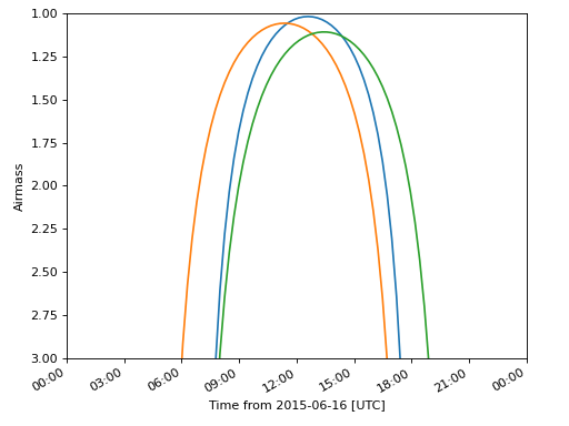
We want a minimum airmass when observing, and it looks like sometime between 9:00 and 15:00 UTC (or 23:00 on the 15th to 5:00 on the 16th, US/Hawaii) would be the best time to observe all three targets.
However, if we want to define a more specific time window based on airmass, we
can calculate this quantity directly. To get airmass measurements, we need to
use the AltAz frame:
>>> subaru.altaz(time, altair).secz
<Quantity 1.0302347952130682>

>>> subaru.altaz(time, vega).secz
<Quantity 1.0690421636016616>

>>> subaru.altaz(time, deneb).secz
<Quantity 1.167753811648361>
Behind the scenes here, subaru.altaz(time, altair) is actually creating
an AltAz object in the AltAz frame, so if you
know how to work with coordinates objects, you can do lots more
than just computing airmass.
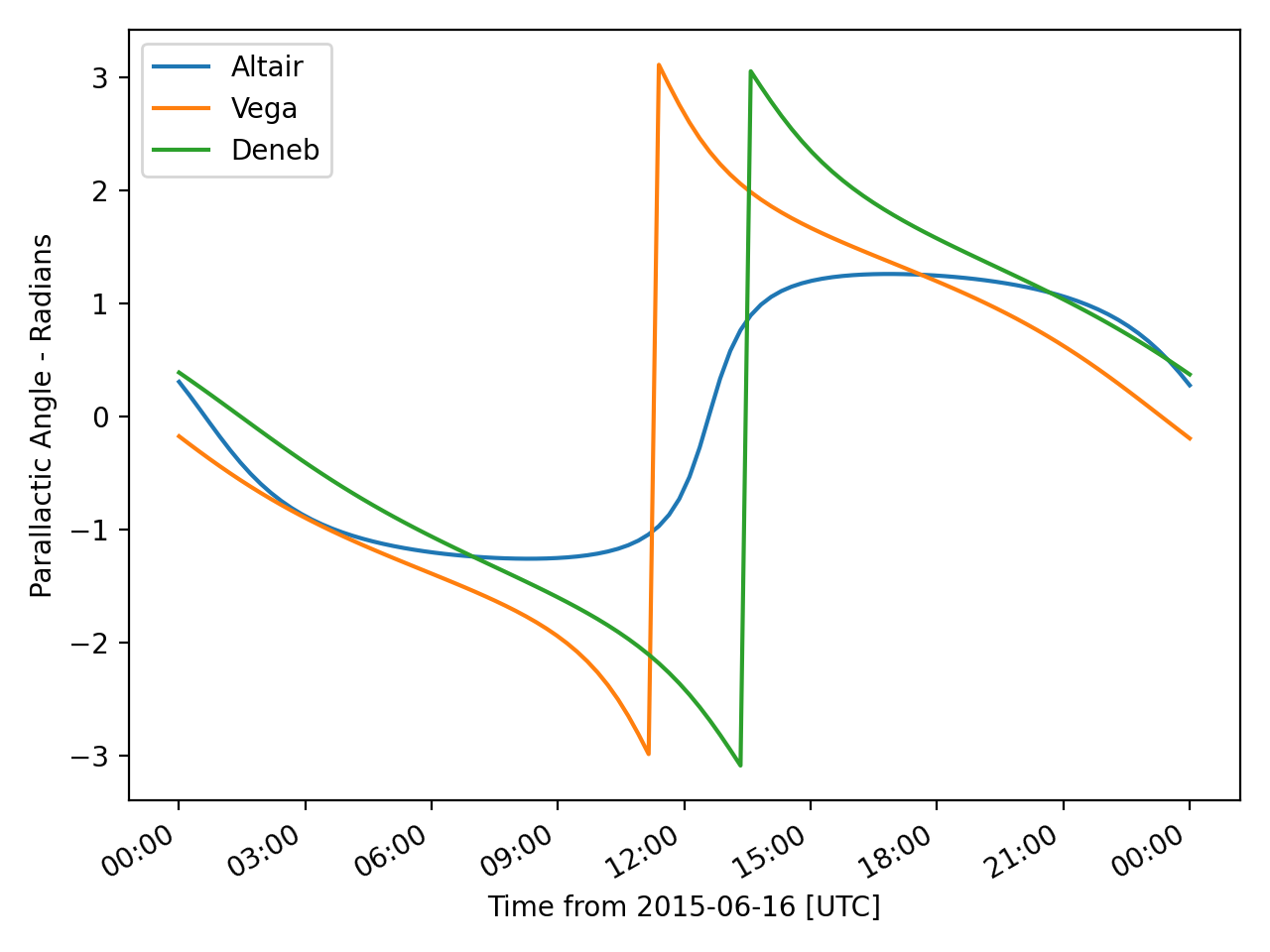
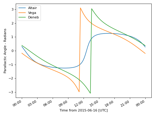
Parallactic Angle#
To get a general idea of our targets’ parallactic angle on the night of observation, we can make another plot (again, see Plotting with Astroplan for more on customizing plots and the like):
>>> import matplotlib.pyplot as plt
>>> from astroplan.plots import plot_parallactic

>>> plot_parallactic(altair, subaru, time)
>>> plot_parallactic(vega, subaru, time)
>>> plot_parallactic(deneb, subaru, time)

>>> plt.legend(loc=2)
>>> plt.show()
(Source code, png, hires.png, pdf, svg)
We can also calculate the parallactic angle directly:
>>> subaru.parallactic_angle(time, altair)
<Angle -0.6404957821112053 rad>

>>> subaru.parallactic_angle(time, vega)
<Angle -0.46542183982024 rad>

>>> subaru.parallactic_angle(time, deneb)
<Angle 0.7297067855978494 rad>
The Angle objects resulting from the calls to
parallactic_angle() are subclasses of the Quantity
class, so they can do everything a Quantity can do -
basically they work like numbers with attached units, and keep track of
units so you don’t have to.
For more on the many things you can do with these, take a look at the
Astropy documentation or tutorials. For now the most useful thing is to
know is that angle.degree, angle.hourangle, and angle.radian
give you back Python floats (or numpy arrays) for the angle in degrees,
hours, or radians.
The Moon#
If you need to take the Moon into account when observing, you may want to know when it rises, sets, what phase it’s in, etc. Let’s first find out if the Moon is out during the time we defined earlier:
>>> subaru.moon_rise_time(time)
<Time object: scale='utc' format='jd' value=2457190.1696768994>

>>> subaru.moon_set_time(time)
<Time object: scale='utc' format='jd' value=2457189.684134357>
We could also look at the Moon’s alt/az coordinates:
>>> subaru.moon_altaz(time).alt
<Latitude -45.08860929634166 deg>

>>> subaru.moon_altaz(time).az
<Longitude 34.605498354422686 deg>
It looks like the Moon is well below the horizon at the time we picked before, but we should check to see if it will be out during the window of time our targets will be visible (again–as defined at the beginning of this tutorial):
>>> visible_time = start + (end - start)*np.linspace(0, 1, 20)

>>> subaru.moon_altaz(visible_time).alt
<Latitude [-25.21127325,-30.68088873,-35.82145644,-40.53415037,
           -44.68898859,-48.12296182,-50.64971858,-52.08946099,
           -52.31849772,-51.31548444,-49.17038499,-46.04862654,
           -42.13887599,-37.61479774,-32.61875342,-27.26048709,
           -21.62215227,-15.76463668, -9.73313141, -2.19408792] deg>
Looks like the Moon will be below the horizon during the entire time.
Sky Charts#
Now that we’ve determined the best times to observe our targets on the night in question, let’s take a look at the positions of our objects in the sky.
We can use plot_sky as a sanity check on our target’s
positions or even just to better visualize our observation run.
Let’s take the start and end of the time window we determined
earlier (using the most basic definition
of “visible” targets, above the horizon when the sun is down), and see where our
targets lay in the sky:
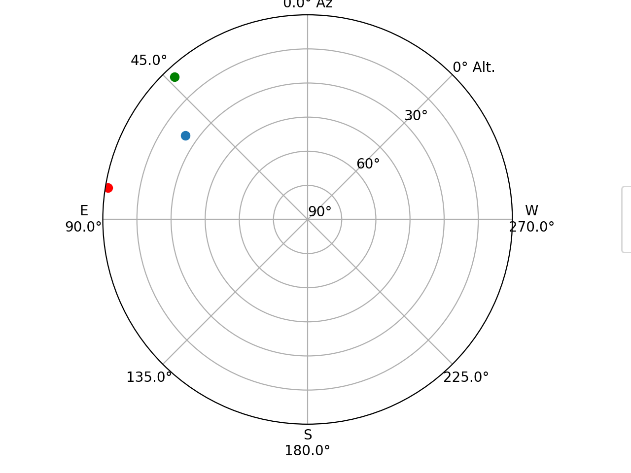
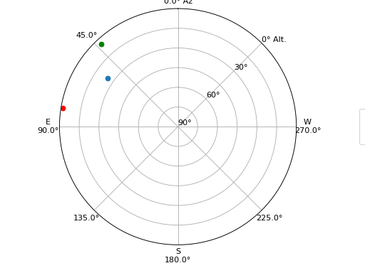
>>> from astroplan.plots import plot_sky
>>> import matplotlib.pyplot as plt
>>> altair_style = {'color': 'r'}
>>> deneb_style = {'color': 'g'}
>>> plot_sky(altair, subaru, start, style_kwargs=altair_style)
>>> plot_sky(vega, subaru, start)
>>> plot_sky(deneb, subaru, start, style_kwargs=deneb_style)
>>> plt.legend(loc='center left', bbox_to_anchor=(1.25, 0.5))
>>> plt.show()
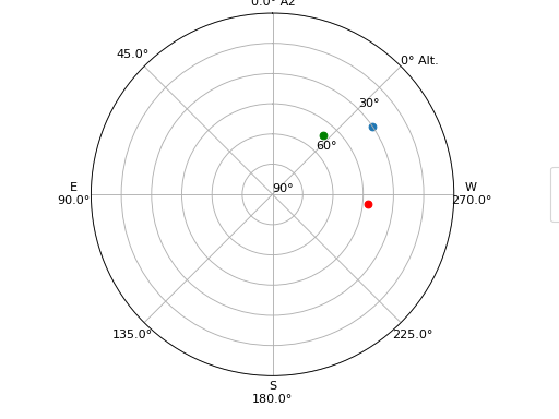
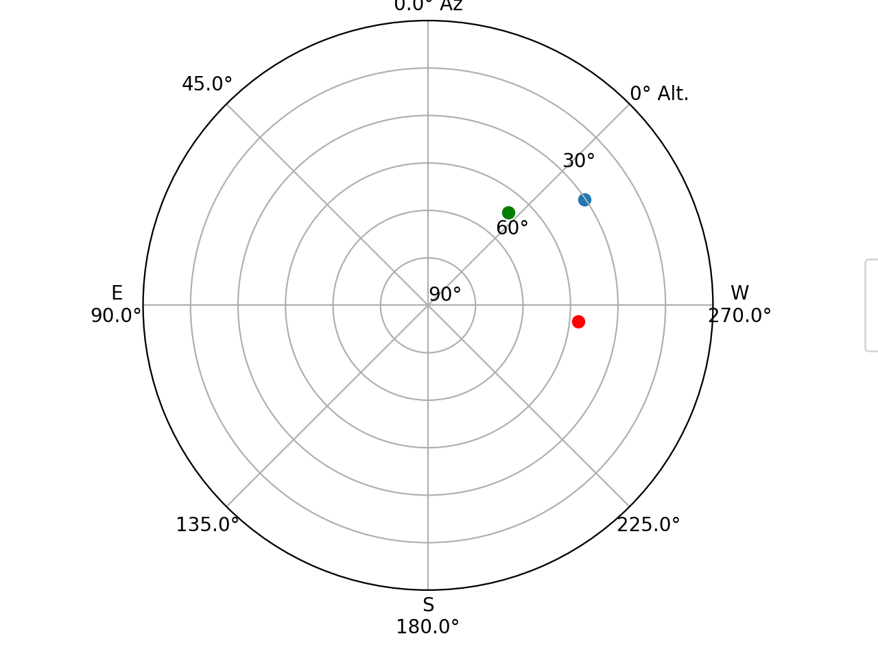
>>> plot_sky(altair, subaru, end, style_kwargs=altair_style)
>>> plot_sky(vega, subaru, end)
>>> plot_sky(deneb, subaru, end, style_kwargs=deneb_style)
>>> plt.legend(loc='center left', bbox_to_anchor=(1.25, 0.5))
>>> plt.show()
(Source code, png, hires.png, pdf, svg)

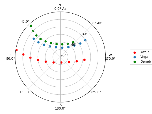
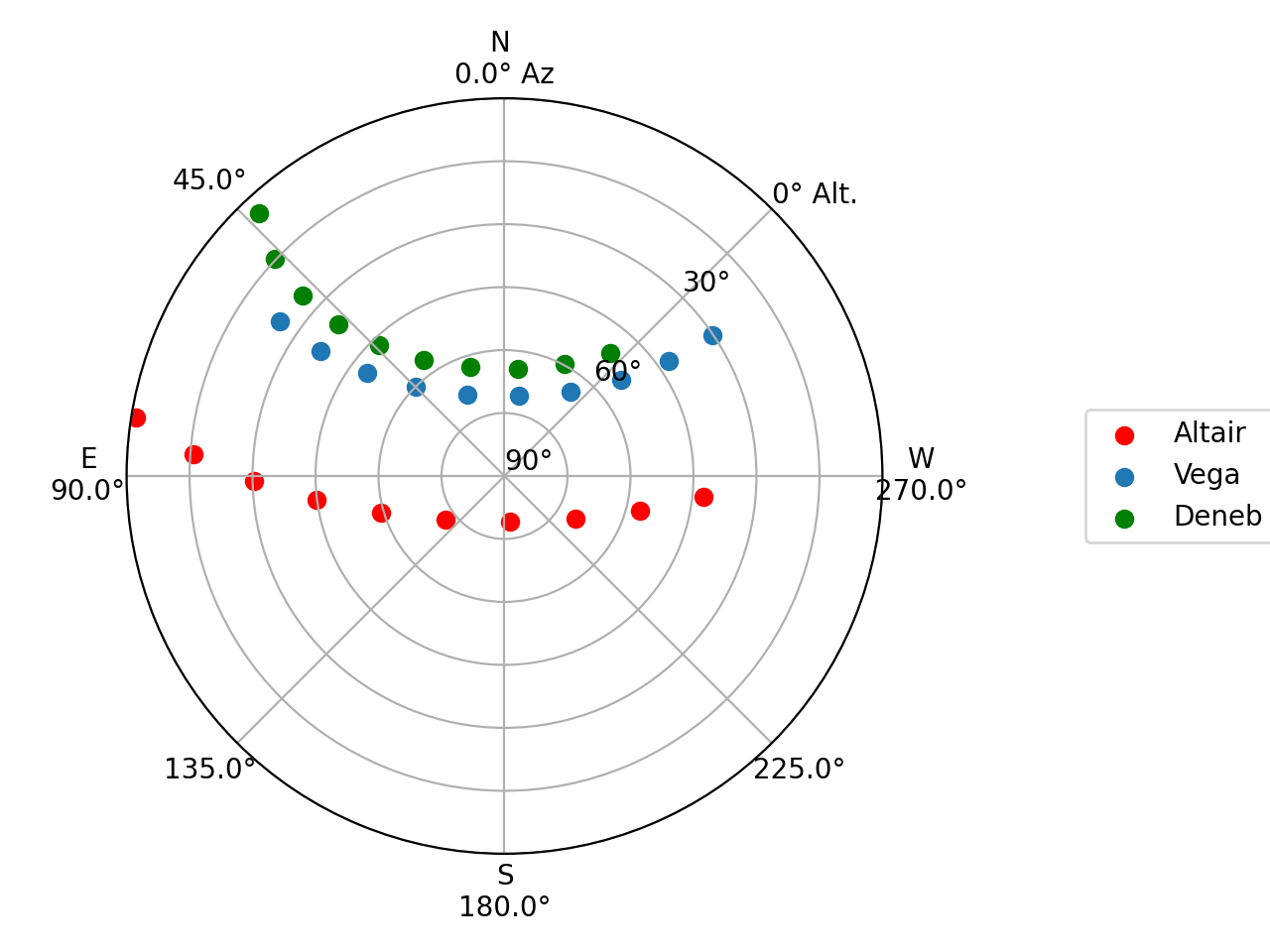
We can also show how our targets move over time during the night in question:
>>> time_window = start + (end - start) * np.linspace(0, 1, 10)

>>> plot_sky(altair, subaru, time_window, style_kwargs=altair_style)
>>> plot_sky(vega, subaru, time_window)
>>> plot_sky(deneb, subaru, time_window, style_kwargs=deneb_style)

>>> plt.legend(loc='center left', bbox_to_anchor=(1.25, 0.5))
>>> plt.show()
(Source code, png, hires.png, pdf, svg)